saeHB.TF.beta provides several functions for area and
subarea level of small area estimation under Twofold Subarea Level Model
using hierarchical Bayesian (HB) method with Beta distribution for
variables of interest. Some dataset simulated by a data generation are
also provided. The ‘rstan’ package is employed to obtain parameter
estimates using STAN.
You can install the development version of saeHB.TF.beta from GitHub with:
# install.packages("devtools")
devtools::install.github("Nasyazahira/saeHB.TF.beta")Here is a basic example of using the betaTF function to make estimates based on sample data in this package
library(saeHB.TF.beta)

#Load Dataset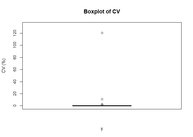
data(dataBeta) #for dataset with nonsampled subarea use dataBetaNSdataBeta$CV <- sqrt(dataBeta$vardir)/dataBeta$y
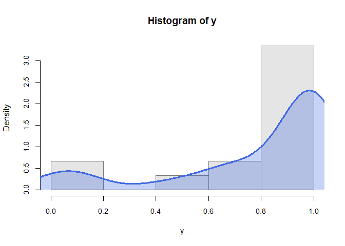
explore(y~X1+X2, CV = "CV", data = dataBeta, normality = TRUE)
#> y X1 X2
#> Min. 0.002826007 0.04205953 0.02461368
#> 1st Qu. 0.677417203 0.34818477 0.20900053
#> Median 0.986658040 0.58338771 0.39409355
#> Mean 0.786269096 0.57240016 0.43864087
#> 3rd Qu. 0.999116512 0.85933934 0.73765722
#> Max. 1.000000000 0.99426978 0.96302423
#> NA 0.000000000 0.00000000 0.00000000
#>
#> Normality test for y :
#> Decision: Data do NOT follow normal distribution, with p.value = 0 < 0.05
#Fitting model
fit <- betaTF(y~X1+X2, area="codearea", weight="w", data=dataBeta, iter.update = 5, iter.mcmc = 10000)Area mean estimation
fit$Est_areaArea random effect
fit$area_randeffCalculate Area Relative Standard Error (RSE) or CV
RSE_area <- (fit$Est_area$SD)/(fit$Est_area$Mean)*100
summary(RSE_area)Subarea mean estimation
fit$Est_subSubarea random effect
fit$sub_randeffCalculate Subarea Relative Standard Error (RSE) or CV
RSE_sub <- (fit$Est_sub$SD)/(fit$Est_sub$Mean)*100
summary(RSE_sub)fit$coefficientfit$refVarlibrary(ggplot2)Save the output of Subarea estimation and the Direct Estimation (y)
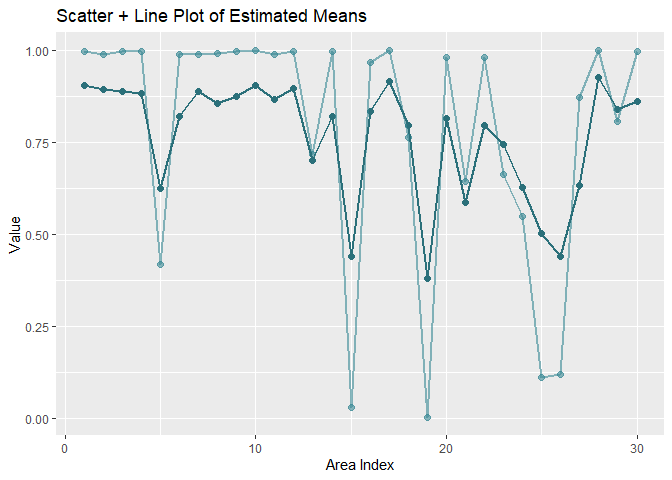
df <- data.frame(
  area = seq_along(fit$Est_sub$Mean),
  direct = dataBeta$y,
  mean_estimate = fit$Est_sub$Mean
)
Area Mean Estimation
ggplot(df, aes(x = area)) +
  geom_point(aes(y = direct), size = 2, colour = "#388894", alpha = 0.6) +   # scatter points
  geom_point(aes(y = mean_estimate), size = 2, colour = "#2b707a") +   # scatter points
  geom_line(aes(y = direct), linewidth = 1, colour = "#388894", alpha = 0.6) +  # line connecting points
  geom_line(aes(y = mean_estimate), linewidth = 1, colour = "#2b707a") +  # line connecting points
  labs(
    title = "Scatter + Line Plot of Estimated Means",
    x = "Area Index",
    y = "Value"
  )
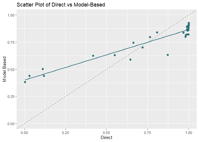
ggplot(df, aes(x = , direct, y = mean_estimate)) +
  geom_point( size = 2, colour = "#2b707a") +
   geom_abline(intercept = 0, slope = 1, color = "gray40", linetype = "dashed") +
  geom_smooth(method = "lm", color = "#2b707a", se = FALSE) +
  ylim(0, 1) +
  labs(
    title = "Scatter Plot of Direct vs Model-Based",
    x = "Direct",
    y = "Model Based"
  )
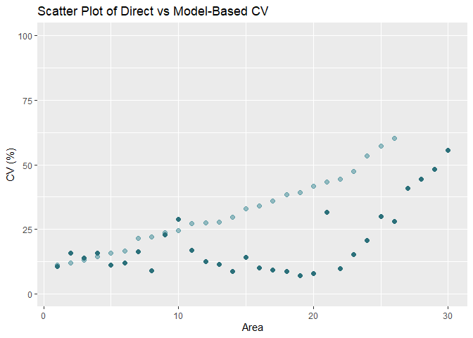
Combine the CV of direct estimation and CV from output
df_cv <- data.frame(
  direct = sqrt(dataBeta$vardir)/dataBeta$y*100,
  cv_estimate = RSE_sub
)
df_cv <- df_cv[order(df_cv$direct), ]
df_cv$area <- seq_along(dataBeta$y)
Relative Standard Error of Subarea Mean Estimation
ggplot(df_cv, aes(x = area)) +
  geom_point(aes(y = direct), size = 2, colour = "#388894", alpha = 0.5) +
  geom_point(aes(y = cv_estimate), size = 2, colour = "#2b707a") +
  ylim(0, 100) +
  labs(
    title = "Scatter Plot of Direct vs Model-Based CV",
    x = "Area",
    y = "CV (%)"
  )